Kyle Shepherd

Music Clustering Project

## Introduction

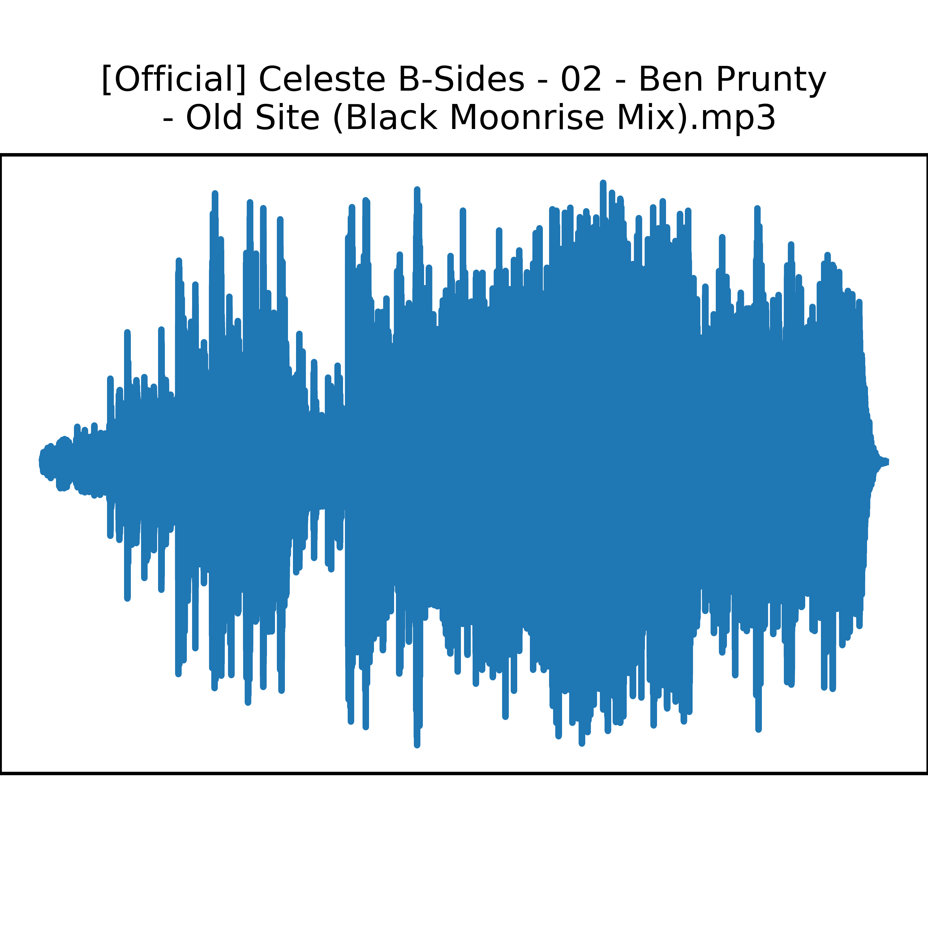
I have collected a personal music collection over the years. I have ~1,800 songs, ~14 GB of music, 157 hours (6.5 days). Most of my music is in the form of mp3 files that I ripped off of YouTube, SoundCloud, bandcamp, etc. As a consequence, my music lacks any kind of identifying metadata. No category data, no artist data, no album data, and the filename does not always match the song title.

Therefore, I do not know what categories of music I have. And existing software to categorize my songs cannot handle the lack of metadata. And online services such as Spotify do not have my songs in their database. Therefore, the only information I have about the song is the actual song itself, the waveform data.

I could attempt to manually label all of my songs. But I know nothing about music theory (I have no musical ear despite playing the trombone for 11 years).

I could place my songs in general categories of piano, orchestral, rock/metal, and electronic, but I could not be more specific than that.

I wanted to determine if I could automatically cluster my song library just using the song waveform data, using my computer to find similar songs. Once the algorithm clusters my music, I can label the cluster myself (peaceful music, exercise music, study music, etc.). With these clusters in hand, I can make playlists, find more of a song I currently like, give similar songs to someone who likes an individual song from my library, and other such tasks.

## Procedure

### Feature Extraction

Overall, this problem can be framed as an unsupervised machine learning problem. Step 1 is to figure out how to compare songs, defining similarity of songs.

One possible method is to just compare the raw waveform data of the songs, the amplitudes. But there are several issues with this approach. One, the data is of variable length so a one-to-one comparison is not possible. Two, songs could have different sample rates, how much data exists per second. Three, the raw amplitude data is noisy and does not directly convey the aspects of music that I like, such as frequencies, tones, harmonics, timbre, beats, tempo, etc. So an algorithm would somehow have to learn these attributes itself, which is a very hard task for a machine to do when all of my data is unlabeled.

 1 import os
 2 from scipy.io import wavfile
 3 
 4 import matplotlib
 5 matplotlib.use('Agg')  # no UI backend
 6 import matplotlib.pyplot as plt
 7 plt.rcParams['agg.path.chunksize'] = 10000
 8 
 9 # set up plotting area
10 plt.rc('xtick', labelsize=6)
11 plt.rc('ytick', labelsize=6) #labelsizes
12 plt.rc('axes', titlesize=8)  #titlesize
13 dx = 3 #plot size in inches
14 dy = 3 #plot size in inches
15 fig = plt.figure(figsize=(dx, dy)) #makes figure/canvas space
16 plot = fig.add_axes([0 / dx, 0.5 / dy, 3 / dx, 2 / dy])
17 
18 folder='../../../Media/Music/'
19 MusicName='[Official] Celeste B-Sides - 02 - Ben Prunty - Old Site (Black Moonrise Mix).mp3'
20 MusicName='Starbound OST - Altair.mp3'
21 filein=folder+MusicName
22 # os.system('ffmpeg -i "'+filein+'" -ac 1 output.wav -y')
23 os.system('ffmpeg -i "'+filein+'" -ac 1 output.wav -y')
24 
25 A=wavfile.read('output.wav')
26 print(A[1])
27 plot.plot(A[1])
28 plot.set_xticks([])
29 plot.set_yticks([])
30 plot.set_title('[Official] Celeste B-Sides - 02 - Ben Prunty\n - Old Site (Black Moonrise Mix).mp3')
31 fig.savefig("Waveform.png",dpi=1000)
32 plot.clear()

Therefore, I need to extract these features from the song before handing it off to an classification algorithm. FFMPEG can convert music files to .WAV, which can be read into a program as a vector of amplitudes. Unfortunately, there is no overall theory to convert the audio waveforms to human subjective values, there is no way to directly measure how "good" a song is. Spotify has a few metrics they measure such as acousticness, danceability, energy, instrumentalness, liveness, speechiness, and valence. [Link to Spotify's documentation](https://developer.spotify.com/documentation/web-api/reference/tracks/get-audio-features/) However, they do not provide details on how to calculate these values, so these metrics are not available unless spotify has the song in their database.

### Spectral Analysis

I can take an approach inspired from spotify and attempt to extract spectral features from my songs. Fortunately, a python package exists that can extract a variety of features. pyAudioAnalysis by tyiannak. [Repo here](https://github.com/tyiannak/pyAudioAnalysis). This package was also used in a paper [pyAudioAnalysis: An Open-Source Python Library for Audio Signal Analysis](https://doi.org/10.1371/journal.pone.0144610). The features available in this package include.

These seem to capture the characteristics of music well, and they use domain knowledge. Mel Frequency Cepstral Coefficients are a very specific set of features well tuned to how humans interpret sounds and music. However, I had some doubts about these features. I could not be sure these would capture all the relevant information about my music collection, so the classification algorithm would not have the data it needs to succeed. And these features still require some "window of analysis", it only inspects short portions of songs. A given song is divided up into N number of windows, and each window will have the feature calculated. So in essence I just convert my raw waveform data into a shorter time series, with all of the same problems as comparing the raw waveform data.

### Alternative Features

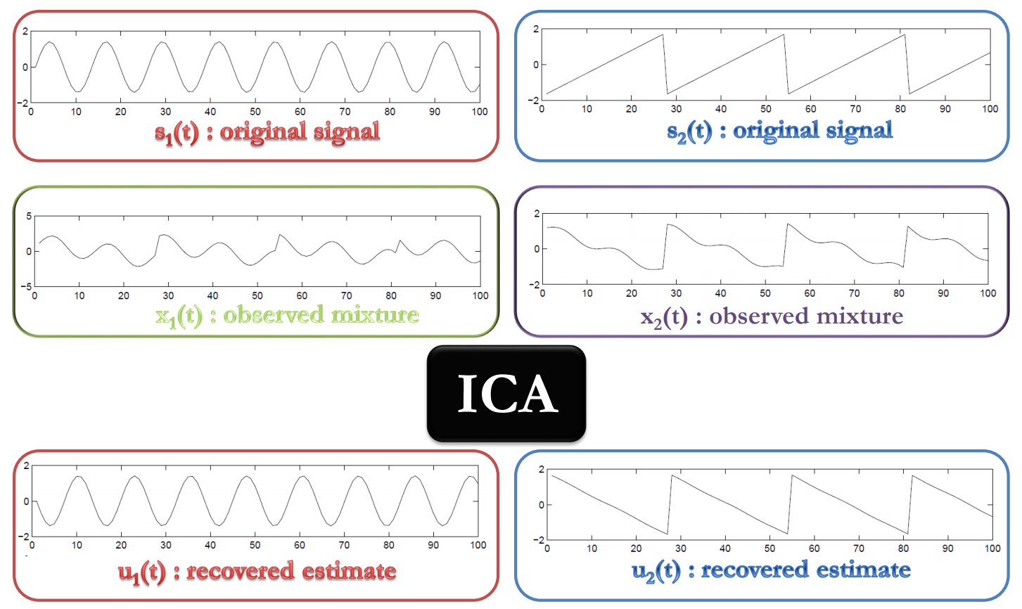
Therefore, I looked at a few alternatives for extracting features from my songs. The first thing I tried was to extract the individual instruments from each song. Getting the instruments of a song is like solving the cocktail party effect. [The figure is from http://www.sci.utah.edu/~shireen/pdfs/tutorials/Elhabian_ICA09.pdf](http://www.sci.utah.edu/~shireen/pdfs/tutorials/Elhabian_ICA09.pdf) Each instrument is like a "speaker", and our brains can separate out individual speakers in a crowd, so an algorithm should be able to do the same thing. While there are sophisticated algorithms out there that can do this, the problem is still an open problem for music, the source separation problem. I do not need state-of-the-art results, I just need something that kind of works, so I tried using Independent Component Analysis. While Independent Component Analysis works for small toy cases (separating sin waves from sawtooth waves), it was an abysmal failure for my use case. The instruments it produced were just noise, no longer recognizable as instruments. This approach was much harder than anticipated, so I just dropped this line of analysis.

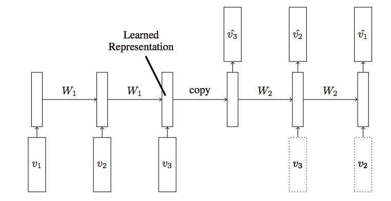
The second alternative I tried was using LSTM Recurrent Neural Networks. [Architecture explained at this link, "A Gentle Introduction to LSTM Autoencoders"](https://machinelearningmastery.com/lstm-autoencoders/) Python packages make building and training simple neural networks easy, so I figured I would try to do the same thing. The architecture I attempted was a Recurrent Neural Network Autoencoder. It would take the song (or the feature time series), output a short vector of ~10 features (compressing the entire song to ~10 variables), then attempt to reconstruct the original song from the short feature vector. The Encoder would learn to output better representations of a song, and the Decoder would learn how to best reconstruct a song. However, this architecture failed on very simple test cases. I gave it 3 linear series of 100 data points. One with a positive slope, one with a negative slope, and one with a zero slope. These lines can be encoded by 2 variables (the starting point, and the slope), so I expected the neutral network to learn this representation, this compression. However, no matter how many variables I allowed the network to output, or which activation units I used (ReLU or Exponential Linear Units), or which gradient decent schemes I used, the neutral net always produced terrible reconstructions of these linear lines. In addition, it started encountering training instability if the time series were described with more than 1000 data points, which means this method would not scale up to analyzing a song with millions of data points. Due to the failure to solve this toy example, I dropped this line of investigation.

### Alternative Features

Due to the failure of the above alternatives, I was back to the spectral features. However, I still had to solve how to convert the time series of features into a single feature vector for an individual song.

One approach is to take statistics of the time series. So I could have the mean, standard deviation, quartile ranges, linear fit coefficients, spline fit coefficients, etc. Many people have complied lists of time series features and created programming packages to extract time series features. tsfresh is an example of a package that can extract time series features. [Documentation here](https://tsfresh.readthedocs.io/en/latest/text/list_of_features.html). And B. D. Fulcher, M. A. Little, N. S. Jones in their paper "Highly comparative time-series analysis: the empirical structure of time series and their methods" [https://doi.org/10.1098/rsif.2013.0048](https://doi.org/10.1098/rsif.2013.0048) made an exhaustive effort to identify as many possible time series features as possible, and train machine learning models to identify the relevant features for a given problem. [Supplementary information describing all the features they used is located here](https://royalsocietypublishing.org/action/downloadSupplement?doi=10.1098%2Frsif.2013.0048&file=rsif20130048supp2.pdf&).

However, to include all of these features would cause an explosion in the number of features to analyze, definitely bringing on a curse of dimensionality. I would risk including noisy useless features, and I have no labeled data to filter out the irrelevant features. And these features will also stray from describing how music actually sounds, so the clustering algorithms would not cluster the music in a meaningful way for me.

### Beat Analysis

To get around all of these issues, I needed a way to remove the temporal nature of my songs. For the most part, I care about how individual sections of the song sound. I care about the notes and measures of the song. I do not care as much about how a song transforms over time. Every song is entirely too unique in how it transforms over time, trying to compare how two songs "change" like each other is a very difficult task, even trying to define the change is difficult. Therefore, I just needed to compare the measures, the beats of a song across other songs.

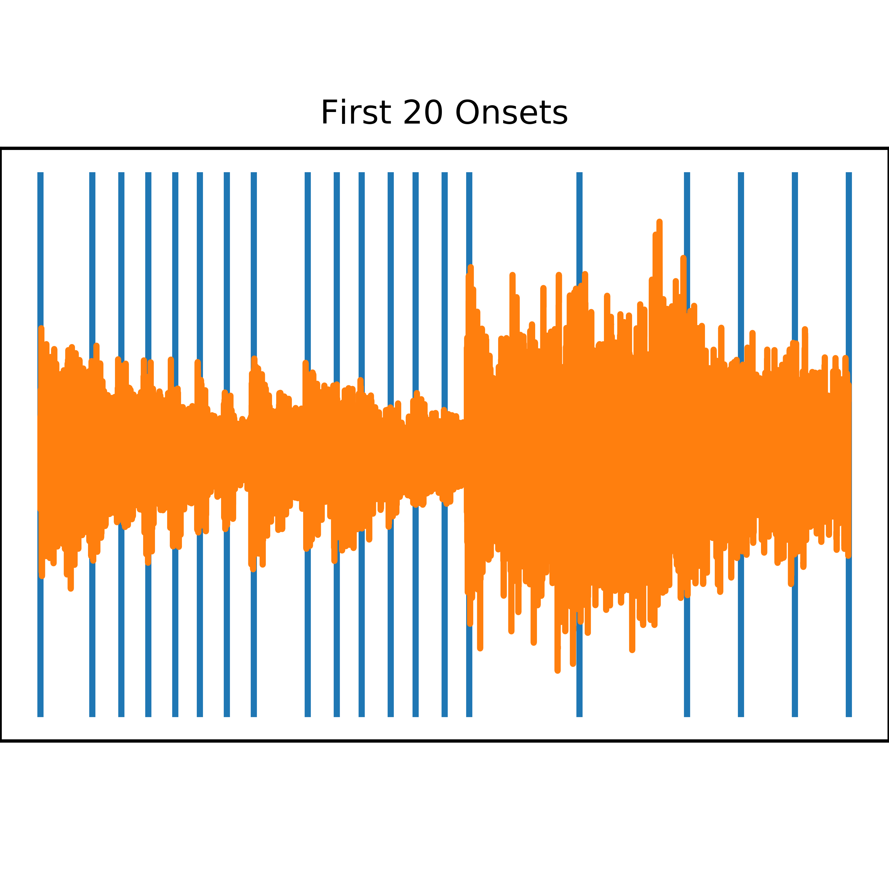
Since the original spectral features require a "window of analysis", I just needed to define my window as a measure or beat of the song. Very fortunately, there are python packages for measuring the beat of a song. While beat detection is in general a hard problem, I just needed "good enough" results. The package librosa has beat detection capabilities. The module [librosa.beat.beat_track](https://librosa.github.io/librosa/generated/librosa.beat.beat_track.html) can identify the beat of a song. As implemented, it is not useful for me, because it identifies one beat for an entire song, when in reality the beat of a song can change over time. However, to find the beat of a song, librosa uses "onset detection", basically finding when notes and measures start. I can just use the raw onset detection results to define the boundaries of my analysis windows.

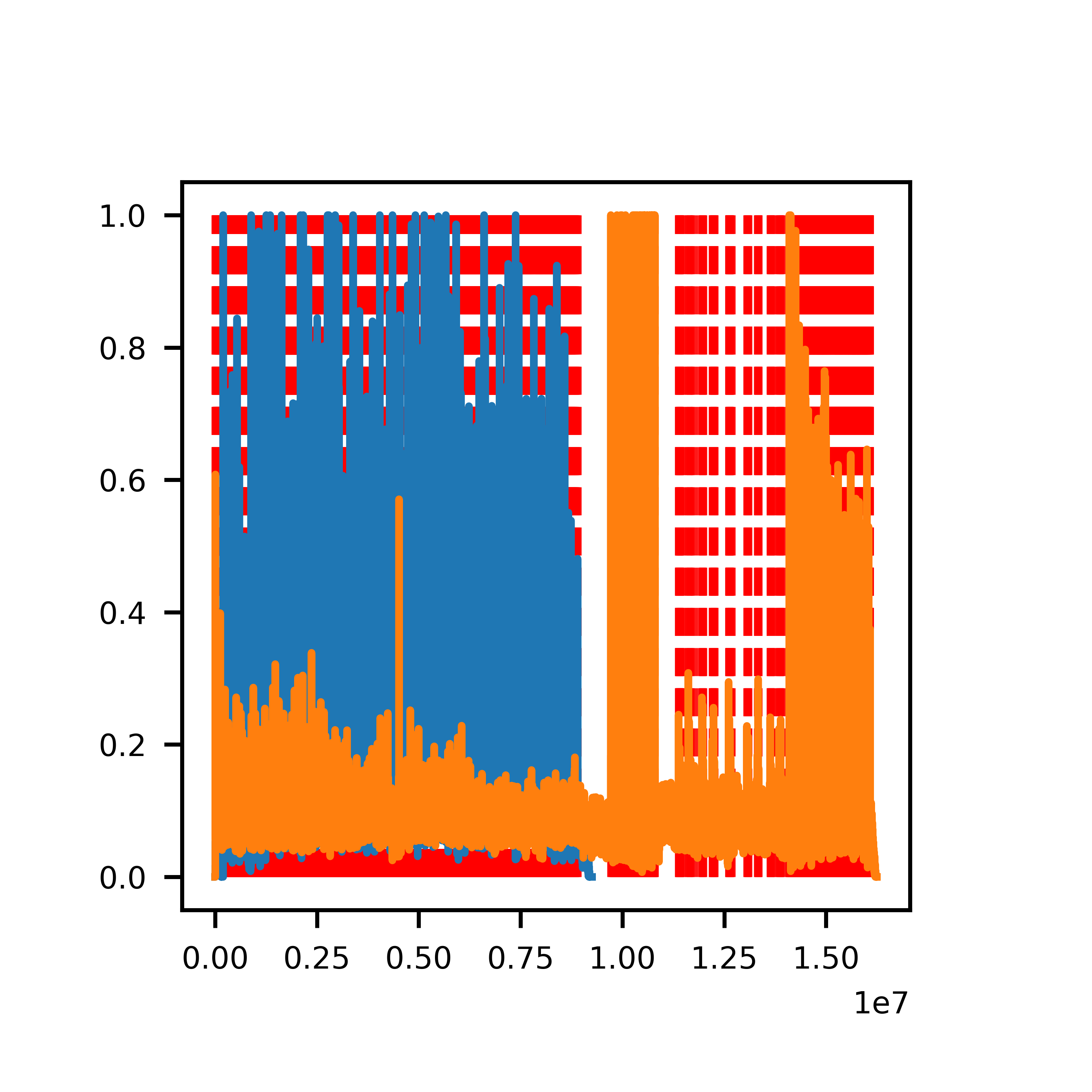
This code calculates the spectral flux across small sized analysis windows, and then finds peak values in the spectral flux values. Newer versions of the analysis code use the backtrack=True keyword in the librosa.onset.onset_detect function. This just backs up the detected onset to a local minimum in the calculated spectral flux value, so that the analysis windows contain the entire onset, and not just half the onset, at the peak. Also, the peak detection algorithm that librosa uses can be sensitive to songs that contain absolute silences, where the spectral flux from the silence to the onset produces large outlier peaks. The peak detection algorithm only detects these large peaks while ignoring other peaks in the song. To solve this problem, I implemented a "peak cutoff" value. Peaks greater than the 99.9% are truncated to the 99.9% value.

 1 import librosa
 2 import numpy
 3 from scipy.io import wavfile
 4 
 5 filename = 'output.wav'
 6 y, sr = librosa.load(filename,sr=None)
 7 beat_frames = librosa.onset.onset_detect(y=y, sr=sr,units='samples')
 8 print(y)
 9 print(y.shape)
10 print(beat_frames.shape)
11 x=[]
12 l=[]
13 st=beat_frames[200]
14 et=beat_frames[219]
15 
16 for b in beat_frames[200:220]:
17     x.append(b)
18     x.append(b)
19     x.append(None)
20     l.append(numpy.min(y[st:et])*1.2)
21     l.append(numpy.max(y[st:et])*1.2)
22     l.append(None)
23 
24 plot.plot(x,l)
25 plot.plot(numpy.arange(st,et),y[st:et])
26 plot.set_title('First 20 Onsets')
27 plot.set_xticks([])
28 fig.savefig("Windows.png",dpi=1000)
29 plot.clear()
30 
31 length=et-st
32 pad=int(length/10)
33 out=numpy.insert(y[st:et],numpy.repeat(beat_frames[200:220]-st,pad),0)
34 wavfile.write('test.wav',sr,out)

### Feature Calculation

Now that I actually know what to calculate and measure from my songs, I can start implementing some code. While writing the code, I had to adjust for some difficulties. First, I have some hour long songs that would encounter processing difficulties, mostly related to running out of memory. I used FFMPEG to split songs into 30 minute segments to avoid this issue. Also, turning the pagefile back on helped the Operating System make room in RAM during the program. Second, I needed to do some sanity checking of the input files, to make sure they are actual music files, and to make sure there are enough detectable beats. I also had to sanity check the analysis windows, to make sure they were large enough widows. Windows that were too short encountered computational issues related to the MFCC computation, and windows that are too short do not sufficiently capture low frequency sounds. Since human hearing can go down to 20 hz, I set the minimum window size threshold as sample rate/20. Short windows are combined with adjacent windows to make one longer window.

I also had to patch the audioFeatureExtraction module. First, I had to edit the stFeatureExtraction function to accept a list of arbitrarily sized windows. Second, one of the features, the spectral flux, calculates a difference across frames, so I had to remove that from the list of calculated features. Third, the variable length windows caused the default numpy fft algorithm to not perform well (I do not think it performs well on almost prime numbers), so I had to use the pyfftw package to replace the behavior of the numpy fft algorithm. I also found some computational inefficiencies when constructing the MFCC filter banks and Chroma matrices, so I was able to accelerate the computations.

This code can process my music collection faster than the playtime of the songs. But it still takes a little while. An overnight run is required to process the library. Most of the processing is single threaded, so spawning more processes can utilize multiple CPU cores and speed up the processing.

From this calculation, I now have a list of ~1.7 (2.7) million vectors describing the beats of my songs. Each vector contains 33 values that describe the individual beat of the song.

### Recommendation Engine

While I now have a vector of numbers that describe my songs, I still need a way to make these vectors useful. The first thing I tried was calculating the euclidian distance between two feature vectors. In theory, beats that are similar to each other should be close in this feature space, this 33 dimensional space. I can find the k nearest neighbors of each beat. These nearest neighbors are "similar" beats, so if I want similar beats recommended to me, knn is a logical way to obtain recommendations.

Recommendations from one beat to another are surprisingly accurate. I have included an audio sample of the 100 nearest beats, an audio sample of far away beats, and an audio sample of the 100 furthest away beats.

The initial beat was the 100th beat of 'Song of Healing' (Majora's Mask) - Vocal Cover by Nicki Jensen [w_ Lyrics].mp3. The close beats are still very piano or vocal. The middle beats are jazzy and not similar. The far away beats are sharp and trancy.

I did perform a little bit of data normalization and weighting. I normalized by subtracting the mean from the data, and then dividing by the standard deviation. Newer versions of the feature engine also transform the data to a more normal distribution. Square root, Cube Root, or log was applied to transform the data to a more normal distribution. Then I weighted the data by reducing the value of the Mel Frequency Cepstral Coefficients and the Chroma Vector. Since there are 13 and 12 values respectively to describe this individual characteristic, I did not want these features to be 13 or 12 times more important than the other features. I wanted to weight it so if every single value of the Chroma Vector was a unit of 1 away, it would be an equivalent Euclidian distance of 1. $$C_{beat i}-C_{beat j}=1$$ and

$$(\sum_{n=1}^{12} (Ci_{v_n}-Cj_{v_n})^2)/weight=1$$

A weight equal to the length of the vector will satisfy this requirement. For computational efficiency, the Mel Frequency Cepstral Coefficients data and the Chroma Vector data was divided by $\sqrt{13}$ and $\sqrt{12}$ respectively.

Getting recommendations from individual beats seems to work well, just by listening to the recommended beats. But if it is used to recommend the next song from the current song, it is a little unstable. Adjacent beats will recommend different songs. To smooth out these results, an "averaged" recommendation can be obtained by getting the 100 recommendations of each beat of the entire song, and then counting the number of times a song is recommended. The most frequently recommended song is the overall recommendation.

Spot checking the results on individual songs, it seems to work well. Song recommendations are within the same genera to my ear. I tend to agree with the recommendations. And the recommendations pass a sanity check, wherein the song is most likely to recommend itself. This means the features are describing actual features of the songs and are not just noise.

### Calculations

This k nearest neighbors approach is useful for finding songs immediately related to a desired song, but runs into some practical issues at the song library scale. To find the k nearest neighbors of a single beat, it has to perform a distance calculation on all 1.7 million (1,700,000) beats. For realistic song recommending, and to perform my clustering analysis, I need to precompute these values. That means performing 1.7 million distance calculations for all 1.7 million beats. That means I need to perform 2.9 trillion (2,900,000,000,000) calculations. In more formal terms, this is an $\mathcal{O}(n^2)$ calculation. If my song library doubles in size, the calculation time increases by a factor of 4.

Fortunately, I was able to run this calculation over the course of a week on a Virtual Private Server hosted by OVH. The server specs were (VPS SSD 1), 2 GHz CPU, 2 GB RAM, 20 GB SSD. I also performed some code optimization using the python numexpr package, to make crunching the numbers easier. (Newer versions of the code use numba). The code can be found at the DistanceCalculations.py module.

### Clustering, Dimensionality Reduction

I originally just wanted to perform k-means clustering on my data to find music categories. However, when I plotted the distributions of the features, they all followed either normal-like distributions or exponential-like distributions. There were no obvious multimodal distributions that k-means could find easily. In addition, when looking at the distributions of distances for a few randomly selected beats, the distances are pretty evenly distributed. This all indicates that the data is relatively uniformly distributed, or at least very diffuse. There are no clear boundaries between categories of music. So that means k-means would not produce meaningful results.

While the knn calculations were running, I attempted some data projection methods, projecting the 33 dimensional space to 2 or 3 dimensions, to attempt to visually find clusters.

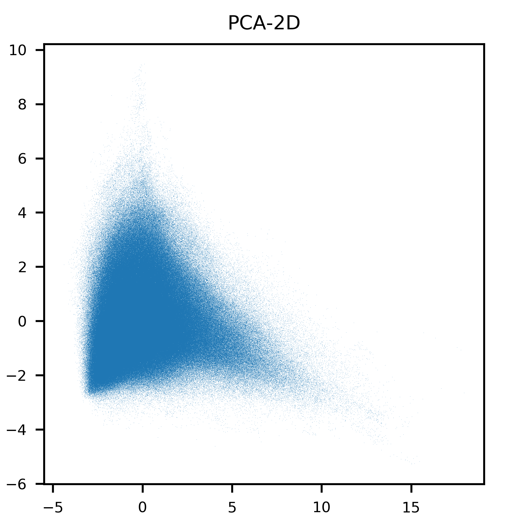
First I tried PCA. As the image shows, it does not result in any clustering in 2D. Even in 3D (Visualized using paraview), it does not result in any clustering.

 1 import numpy
 2 from sklearn.decomposition import PCA
 3 # loads the feature vector from the file we created
 4 data=numpy.load('MusicFeatureData.npy')
 5 
 6 # perform data normalization
 7 mean=numpy.mean(data,axis=0)
 8 std=numpy.std(data,axis=0)
 9 data=(data-mean)/std
10 
11 # perform data weighting
12 s13=numpy.sqrt(13)
13 s12=numpy.sqrt(12)
14 weights=1/numpy.array([1.,1.,1.,1.,1.,1.,1.,s13,s13,s13,s13,s13,s13,s13,s13,s13,s13,s13,s13,s13,s12,s12,s12,s12,s12,s12,s12,s12,s12,s12,s12,s12,1.])
15 data=data*weights
16 
17 x=data
18 pca = PCA(n_components=2)
19 y=pca.fit_transform(x)
20 
21 import matplotlib
22 matplotlib.use('Agg')  # no UI backend
23 import matplotlib.pyplot as plt
24 plt.rcParams['agg.path.chunksize'] = 10000
25 
26 # set up plotting area
27 plt.rc('xtick', labelsize=6)
28 plt.rc('ytick', labelsize=6) #labelsizes
29 plt.rc('axes', titlesize=8)  #titlesize
30 dx = 3 #plot size in inches
31 dy = 3 #plot size in inches
32 fig = plt.figure(figsize=(dx, dy)) #makes figure/canvas space
33 plot = fig.add_axes([0.25 / dx, 0.25 / dy, 2.5 / dx, 2.5 / dy])
34 plot.plot(y[:,0],y[:,1],'o',markersize=0.1,fillstyle='full',markeredgewidth=0.0)
35 plot.set_title('PCA-2D')
36 fig.savefig("PCA-2D.png",dpi=600)
37 plot.clear()
38 
39 pca = PCA(n_components=3)
40 y=pca.fit_transform(x)
41 
42 file=open('paraview.vtk','w')
43 file.write('# vtk DataFile Version 1.0\n')
44 file.write('Power Voronoi\n')
45 file.write('ASCII\n\n')
46 file.write('DATASET POLYDATA\n')
47 file.write('POINTS '+str(y.shape[0])+' float\n')
48 for k in range(0,y.shape[0]):
49     file.write(str(y[k,0])+' '+str(y[k,1])+' '+str(y[k,2])+'\n')
50 file.write('\n')
51 file.close()

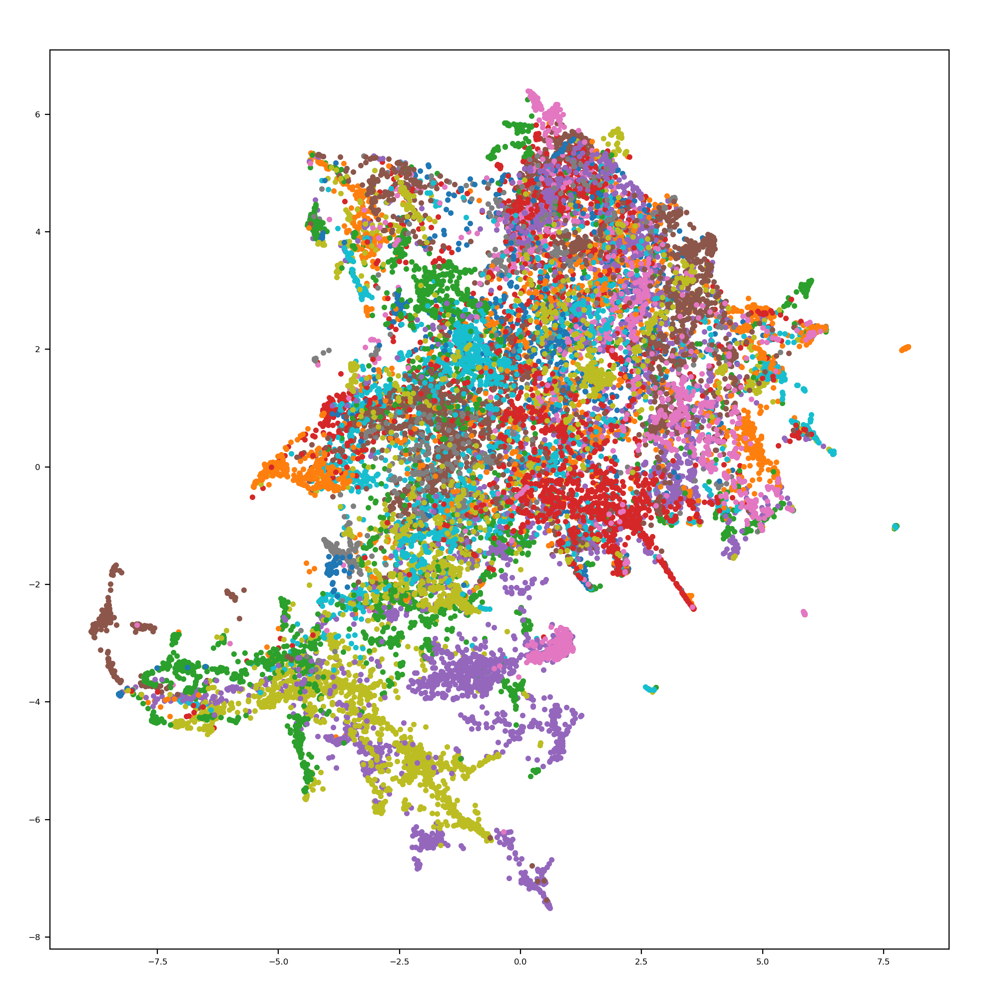
I looked into using t-SNE. However, all of the implementations I could find choked on the 1.7 million data points. I also looked into using UMAP. While it is faster to run, the current implementations choke on the knn calculation, the thing that is taking me a week to run. An example of UMAP on a smaller subsection of my data is shown.

### Clustering, Graph Methods

With the 100 nearest neighbors of all of my beats in hand, I could begin to perform clustering analysis on my songs. The k nn format forms a graph, a network, because it shows relationships between beats. An edge is present if beats are close, no edge otherwise.

The simplest way to try to see clusters is to use graph layout algorithms. The program Gephi has a selection of built in layout algorithms. [Descriptions of the algorithms can be found here.](gephi-tutorial-layouts.pdf) To deal with millions of nodes, only two algorithms can be used. Force Atlas 2 and OpenOrd, because they have complexity scaling of $\mathcal{O}(n*log(n))$. However, Gephi itself is not capable of handling the 1.7 million node network, the program crashes.

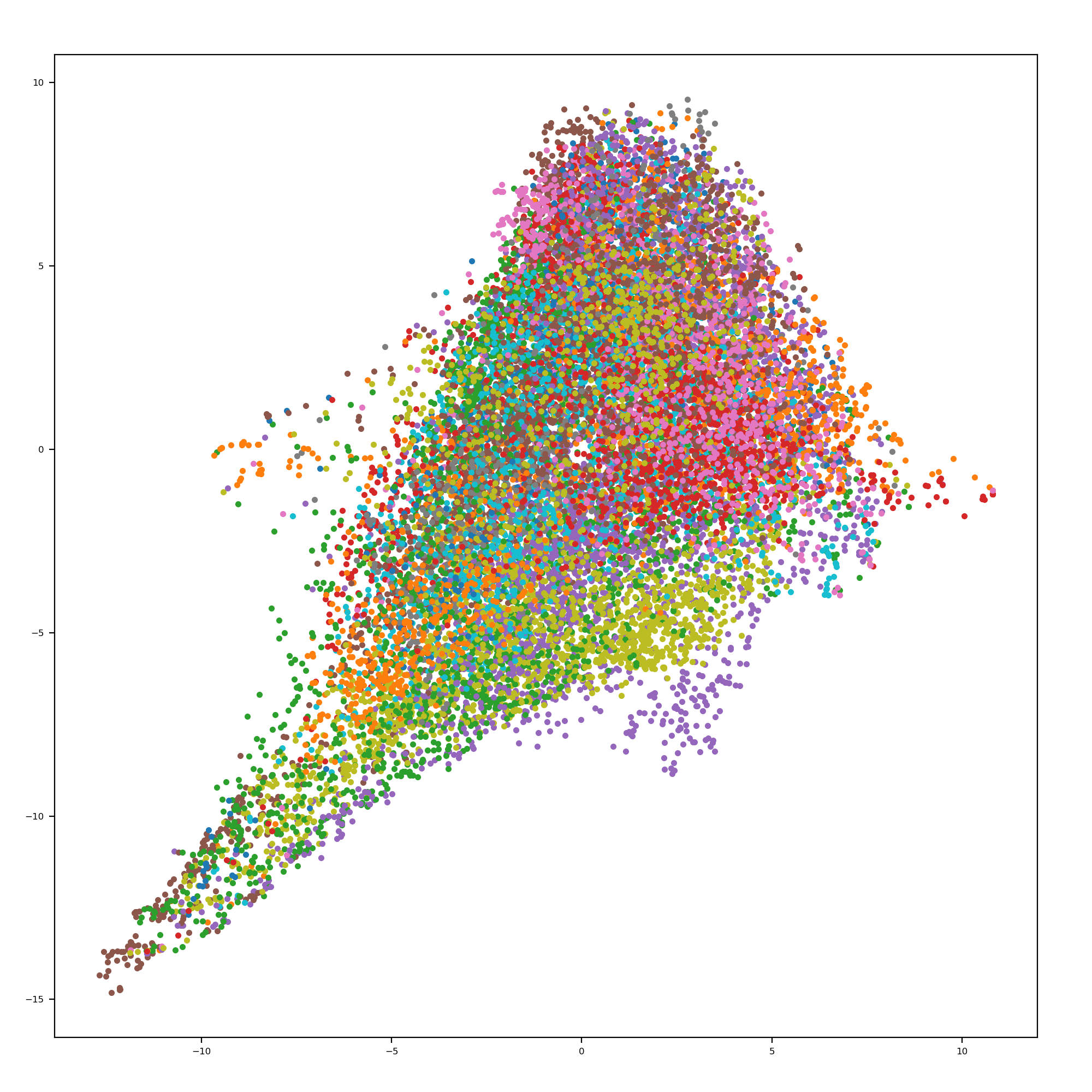
I made a simple implementation of Force Atlas 2, where nodes are attracted to their neighbors, and repelled from the center. It can also produce 3D visualizations. The running time, given the knn or the edges already, is $\mathcal{O}(n*k*\delta)$ where $k$ is the number of knn to consider, and $\delta$ is the number of timesteps to run. The image shows this algorithm running on a 5% subset of beats. Each color is a separate song. While the algorithm seems to work well, comparable results to UMAP, if the songs were not labeled it would not be possible to visually see clusters. Also, it becomes an undifferentiated mess when more data points are added.

 1 import numpy
 2 import ForceLayout
 3 adj=numpy.load('../Alicia Music/adj.npy')
 4 knn=5
 5 adj=adj[:,:knn]
 6 c=numpy.random.rand(adj.shape[0],3)*10
 7 adjmat=numpy.zeros((adj.shape[0],knn+1))
 8 for k in range(0,adj.shape[0]):
 9     adjmat[k,0]=knn
10     adjmat[k,1:]=adj[k,:]
11     # adjmat[k,0]=len(adj[k])
12     # adjmat[k,1:1+len(adj[k])]=adj[k]
13 adjmat=adjmat.astype('uint32')
14 for k in range(0,10):
15     c=ForceLayout.layout3D(adj,c)
16 
17 file=open('paraview.vtk','w')
18 file.write('# vtk DataFile Version 1.0\n')
19 file.write('Power Voronoi\n')
20 file.write('ASCII\n\n')
21 file.write('DATASET POLYDATA\n')
22 file.write('POINTS '+str(y.shape[0])+' float\n')
23 for k in range(0,y.shape[0]):
24     file.write(str(y[k,0])+' '+str(y[k,1])+' '+str(y[k,2])+'\n')
25 file.write('\n')
26 file.close()

### Song Pre-Clustering

Trying to perform any kind of clustering or analysis on these ~2 million datapoints is running into computational limits. The solution to this problem is to pre-cluster the beats of each song. Songs have a repetitive structure, which means many beats should be very similar to each other. The goal is to find "motifs" in a song. Then song recommendations and song clustering can use these motifs instead of individual beats, significantly reducing the computational burden.

To perform this pre-clustering, the MCL algorithm is used. I am using the implementation from [https://github.com/GuyAllard/markov_clustering](https://github.com/GuyAllard/markov_clustering) This algorithm was selected because it has tunable parameters, so the number of identified clusters can be adjusted. Also, its computational complexity is $\mathcal{O}(n^2)$ because it can operate on sparse matrices, so it is fast compared to other clustering algorithms.

MCL performs its clustering on a similarity matrix. The similarity matrix is calculated by finding the 3 nearest neighbors of each beat in the song, calculating the Euclidian distance, and then taking the inverse of the distance. The default pruning value of 0.001, pruning frequency of 1, and expansion value of 2 are used. The inflation value is set to produce the least number of clusters, where no cluster contains more than 10% of the beats. To find this inflation value, a bisection search algorithm is used. Typically 10 iterations of the MCL algorithm using bisection search is needed to find the inflation value.

The feature value of a cluster is taken as the average value of the feature for all the beats in the cluster.

I had some issues running the MCL algorithm implemented by GuyAllard. It had issues clustering the larger songs with ~20,000 beats. I traced the problem down to inefficient handling of scipy sparse matrices. Removing values below a threshold was slow, and the elementwise power function was inefficient. I was able to patch the MCL implementation to speed up the calculations significantly.

I also attempted to program an efficient sparse matrix product algorithm in numba for a performance gain. I assumed the scipy algorithms would have more overhead because they are more general purpose, but the scipy algorithms are actually very optimized, I was only able to get within a factor of 2 of the scipy implementations.

Overall, performing the song pre-clustering is about as fast as extracting all of the beat features, so there is not a large performance penalty for the pre-clustering. On average, there are ~40 beats in a motif. Therefore, when the knn calculations are performed for the motifs, there is a ~1600 factor speedup compared to the beat knn calculation.

### Song Recommendation Engine

Motif-to-motif (MTM) recommendations can be performed similarly to beat-to-beat recommendations. For each motif of a song, the 32 nearest neighbors of a motif can be calculated, and then the number of times the motif of a song is a neighbor can be summed up to generate a song recommendation. However, a few complications arose during the recommendation engine programming.

First, many songs have a "silence" motif. So the silence motif of song A can recommend the silence motif of song B, even if song A and B are very different from each other. To solve this problem, I ignore songs that are only recommended by a single motif.

Second, the MCl algorithm does not guarantee that motifs are close in size to each other. Therefore, motifs with only a few beats have the same recommendation power as a motifs with many beats. This causes recommendations to be sensitive to how MCL decides to split up sub-motifs. The solution is to weight the motifs by the number of beats it contains. First each motif is weighted by $MW=\frac{\text{\# of beats in motif}}{\text{\# of beats in song}}$. Then the motif weights are normalized so the square root of the sum of squared motif weights for a song is equal to 1. $MW_n=\frac{MW}{\sqrt{\sum_{i=1}^{\text{motifs in song}}{MW_i^2}}}$. Finally, the strength of recommendation is obtained by $\text{Motif A weight} * \text{Motif B weight}$.

Therefore, if a motif with lots of beats recommends another motif with lots of beats, the recommendation strength is high. With these changes, the 32 nearest neighbors of each motif of a song are determined, the weight of each connection is calculated, and then the weighted sum of connections to neighboring motifs of a song is used to obtain recommendations.

Once normalized, the MTM recommendations result in a weighted probability vector. When repeated for every song, a stochastic matrix is created, describing a probabilistic chain of recommendations.

Overall, the quality of MTM recommendations appears to be unchanged compared to the beat-to-beat recommendations. While similar songs are recommended based on my ear and opinion, it is difficult to validate the quality of these recommendations without labeled data.

### Song Recommendation Validation

While the quality of MTM recommendations seems good to my ear, I need some way of validating the recommendations. Therefore, I need some form of labeled data. Fortunately, there are databases of royalty-free music that are easy to download, and some of them come with music tags. The database of royalty-free music I ended up using is from Kevin MacLeod at Incompetech. There are ~1400 songs, and most of them are apparently tagged by Kevin MacLeod himself. Tag categories can be seen in the below table. In these categories, there are 436 unique tags.

Kevin MacLeod's music is widely used. On imdb as of April 30, 2020, he has 3282 credits, and his music is used in countless youtube videos.

The Kevin MacLeod dataset has tagged data, so recommendations can be generated from these tags. Given song X, a recommendation system should recommend a song with similar tags. Because the presence or absence of a tag is binary, a bag-of-words approach can be used. We know the total number of tags in the dataset, $T_n$, so each song $s$ is assigned a vector $VT^s$ with $T_n$ elements, with the $n^th$ value set to 1 if the song is tagged with the $n^th$ tag.

A common way of computing similarity between bags-of-words is to compute the cosine similarity.

$$S = \frac{\sum VT^{s1}_i*VT^{s2}_i}{|VT_{s1}|*|VT_{s2}|}$$

The top n recommendations can be obtained by choosing the n songs with the highest cosine similarity. On average, a song has non-zero similarity with 440 songs.

To evaluate a recommendation system against this ground truth data, the goal is to generate a set of song recommendations from song X with the highest average similarity to song X. Due to the variable motif sizes, MTM recommendations are weighted. Therefore, a weighted average similarity to song X will be calculated.

To evaluate the performance of the MTM recommendations, it will be compared against two other recommendation algorithms. Algorithm one will be random recommendations. Algorithm two will be a publicly available state-of-the-art content-based automatic music tagging, MUSIIO. Cosine similarity will be used to generate recommendations from the automatic tagging. During the comparison, the same number of recommendations will be produced by each algorithm.

For the random recommendations algorithm, it is assumed that n songs are randomly chosen from the Kevin MacLeod database. We can directly calu

When comparing the MTM recommendations against the MUSIIO recommendations,

After this project was started, a service called MUSIIO was created. They claim to automatically tag music from the waveform data, and not from metadata or fingerprinting and database lookup. They offer free and real time music tagging at https://www.musiio.com/tag#demo. Using this service with browser automation, song tags were generated for the Kevin MacLeod dataset.

15 Songs longer than 30 minutes were not able to be processed by MUSIIO due to timeout limits.

A total of 380 unique tags were generated by MUSIIO. These tags fall into 18 categories.

Like the Kevin MacLeod tags, the cosine similarity of the MUSIIO automatically generated tags can be calculated. MUSIIO also outputs a "score" number from 0 to 100 for each generated tag. This score reflects either the confidence of the tag, or the percentage of the song that the tag applies too. Therefore, instead of a binary tag vector, a weighted sparse vector is used to represent the tags of a song. The cosine similarity of this sparse vector is calculated.

However, the "CONTENT TYPE" of nearly every song is "music", so nearly every song has non-zero similarity to every other song. To generate a recommendation list, a non-zero similarity threshold can be used.

### Song Clustering Engine

While the Recommendation Engine is unreasonably effective, it does not solve the original problem I had with my music library, which is the lack of organization and groups. Therefore, I want to build a clustering algorithm from the Recommendation Engine. From the Recommendation Engine a weighted directed graph of song recommendations can be constructed. Therefore, the problem reduces to clustering a weighted directed graph. To start building an algorithm to cluster this graph, I need to define the types of clusters I want to find.

Assuming I have n clusters in my music library, I want my songs to be clustered to maximize the strength of recommendations within the cluster, and minimize the number of songs in a cluster that do not recommend each other. Unfortunately, I believe this is an NP-hard problem, I cannot find the optimum solution unless I try every possible combination of song to group assignments. Therefore, I will just have to approximate the solution.

While the MCL algorithm works well for the pre-clustering, it does not work as well for the music library clustering. The main drawback is the inability to control relative group sizes, so the obtained clusters tend to be ***

Also, empirically, the clusters found by MCL are poor (Give example here)

In the above section, I looked at using graph layout algorithms and projection algorithms to cluster the graph of music recommendations from beat-to-beat recommendations. However, none of these algorithms revealed any clear structure or clustering so they are unlikely to work on the graph of music recommendations from motif-to-motif recommendations.

The clustering algorithm that ended up working is a hierarchical clustering algorithm. The specific algorithm used is a bottom-up agglomerative algorithm with an intermediate greedy optimization step inspired from Louvain modularity. When designing this algorithm, I preferred deterministic greedy algorithms instead of randomized algorithms, so the identified song clusters are consistent.

The first step is to assume all songs are in their own cluster. Next is to try all possible 2-cluster mergers, and select the merge that has the best score, strongest internal recommendations. This reduces the number of clusters by one. Then try swapping each song into another cluster, and perform the swap that creates the best score improvement. Repeat swaps until there is no score improvement option remaining. This greedy swap process optimizes the N remaining clusters.

Repeat the merge and swap process until all clusters have been merged into one cluster. Now it is possible to travel up and down the hierarchical clustering, and find the optimal clusters assuming N clusters of songs.

However, determining the real number of clusters is difficult, and the score function used to generate the clusters tends to equalize the size of each cluster at each level. So selecting one level, a number N of clusters, will be wrong if the "true" clustering has clusters of different sizes.

The solution is to take every cluster generated in the hierarchical clustering process, and sort them from best to worst internal score. It is reasonable to assume the best cluster should receive a label, it is a true cluster, a true genre. Every song in this cluster receives this label. These labels are vectors of length h, where h is the number of clusters. This first label is 1 in the first entry, and zero everywhere else, l[0]=1.

Going down the sorted list of clusters, the label vector of the kth cluster is obtained by summing each song's label vector (if the song has already been labeled). If the song has not been labeled, it contributes a vector of l[k]=1 to the sum. The label vector is normalized to a sum of 1. This label vector is assigned to all unlabeled songs in the cluster. In this fashion, songs "inherit" labels from songs already labeled from stronger, better, clusters.

Now song clusters can be identified by determining the most common labels. Finding the greatest sums along the kth dimension can identify clusters, songs related to each other.

The final step is to listen to the songs in the identified clusters, and assign a human name to the identified cluster. Such as naming cluster 10 as "Metal".